Generic small area estimation
Peter Gao and Jon Wakefield
2025-01-03
Source:vignettes/articles/web_only/small-area-estimation.Rmd
small-area-estimation.RmdIn this vignette, we illustrate the use of the
smoothArea and smoothUnit functions for
generic small area estimation of outcomes other than under-five
mortality rates. Using example data presented in the sae
vignette, we compare our results from SUMMER with those
obtained using the sae package (for a survey of other
packages for small area estimation, see Kreutzmann et al. (2019)).
Preliminary
First, we load the necessary packages and data. The required package
INLA is not available via a standard repository, so we
include code for installation if it is not found. The
survey package will be used to generate direct estimates,
while dplyr and tidyr will be used for data
manipulation.
Area level models
Artificial poverty rate example
In their vignette for the sae package, Molina and Marhuenda (2015) generate an
artificial dataset on income and other related variables to illustrate
the use of area level models. In this example, the objective is to
estimate prevalence of poverty in Spanish counties.
data("incomedata")
data("sizeprov")
data("sizeprovedu")
povertyline <- 0.6 * median(incomedata$income) # 6557.143
incomedata$in_poverty <- as.integer(incomedata$income < povertyline)
The incomedata data frame contains information on 17199
observations of individuals in 52 Spanish provinces. Income values and
sampling weights are provided for each individual along with covariate
information including age group and education level. Molina and Marhuenda (2015) define the poverty
line and calculate an indicator variable (which we name
in_poverty) with value 1 if the corresponding income value
is below the poverty line and 0 otherwise.
Direct estimation with sae
Before considering model-based methods for small area estimation, we
compute direct weighted estimators for the desired small area means. The
sae::direct function computes the Horvitz-Thompson
estimator of domain means given by
where
is the population size of domain
,
is the set of sampled observations in domain
,
is the sampling weight for unit
,
and
is the observation for unit
,
for all
.
The sae::direct function also estimates standard deviation
and coefficient of variation for each domain. Note that
is assumed known and is provided in the data frame
sizeprov. The domains of interest are identified via the
provlab variable.
Direct estimation with survey
We can similarly use the survey::svyby function to
compute the Horvitz-Thompson estimates:
incomedata$pop <- sum(sizeprov$Nd[match(incomedata$provlab, sizeprov$provlab)])
design <- survey::svydesign(ids = ~1, weights = ~weight,
                            data = incomedata, fpc = ~pop)

# estimate area totals
svy.DIR <- survey::svyby(~in_poverty, ~provlab, design, svytotal)

# calculate corresponding area mean estimates
svy.DIR$prov_pop <- sizeprov$Nd[match(svy.DIR$provlab, sizeprov$provlab)]
svy.DIR$Domain <-svy.DIR$provlab
svy.DIR$Direct = svy.DIR$in_poverty/svy.DIR$prov_pop
svy.DIR$SD= svy.DIR$se/svy.DIR$prov_pop
Basic area level model
The basic area level model, also called the Fay-Herriot model, treats direct estimates of small area quantities as response data and explicitly models differences between areas using covariate information and random effects Fay and Herriot (1979). The Fay-Herriot model can be viewed as a two-stage model: in the first stage, a sampling model represents the sampling variability of a direct estimator and in the second stage, a linking model describes the between area differences in small area quantities.
Sampling model:
Let be a direct estimator of an area level mean or total . The sampling model treats as a noisy observation of the true finite population quantity :
where is the known sampling variance of the direct estimator .
Linking model:
where (between-area residual variance) is estimated. In this basic Fay-Herriot model, the area-specific random effects are assumed to be independent and identically distributed (IID) between areas.
Below, we provide a quantile-quantile plot comparing the direct estimates to a Gaussian distribution. Here the observed quantiles align well with those from a Gaussian distribution, which lends some support to the basic IID model.
par(pty = "s")
mu.DIR <- mean(sae.DIR$Direct)
sd.DIR <- sd(sae.DIR$Direct)
qqnorm((sae.DIR$Direct - mu.DIR) / sd.DIR, main = "")
abline(0, 1, col = "red")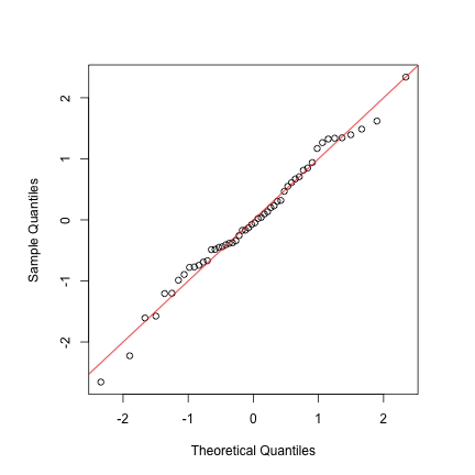
Area level modeling with sae
As described by Molina and Marhuenda
(2015), the sae::mseFH function fits the basic area
level model (via REML by default) and calculates the empirical best
linear unbiased predictors (EBLUP) for all domain means as well as their
estimated MSEs.
sae.FH <- sae::mseFH(sae.DIR$Direct~1, sae.DIR$SD^2)
sae.FH.table <- data.frame(
  Domain = sae.DIR$Domain,
  EBLUP = sae.FH$est$eblup,
  RMSE = sqrt(sae.FH$mse)
)
head(sae.FH.table)
##     Domain      EBLUP       RMSE
## 1    Alava 0.23407448 0.03836098
## 2 Albacete 0.15335213 0.02744856
## 3 Alicante 0.20511853 0.02051886
## 4  Almeria 0.24498009 0.03427432
## 5    Avila 0.07797403 0.02372809
## 6  Badajoz 0.20928033 0.02186672
Area level modeling with SUMMER
The SUMMER package adopts a Bayesian approach to
inference using models such as the basic area level model, carrying out
computation via the INLA package. The
smoothArea function computes direct estimates and then
produces smoothed estimates using a Bayesian Fay-Herriot model. The main
arguments of interest are:
-
formula: Describing the response variable and any area-level covariates -
domainA one-sided formula with the variable containing domain labels on the right. The domain labels variable should be contained in the dataset used to generate the design. -
design: Asurvey.designobject containing survey data and specifying the survey design.
In addition, other commonly used optional arguments include:
-
adj.mat: Optional adjacency matrix if a spatial smoothing model is desired. -
transform: If"logit"is specified, a logit transform will be applied to the direct estimates and an appropriate transformation will be applied to the estimated sampling variances before smoothing. -
direct.est: The direct estimates may be specified directly and smoothing will be applied directly to these user-provided estimates. -
X.domain: Data frame of area level covariates. -
domain.size: Data frame of domain sizes used for computing direct estimates if domain sizes are known.
Other optional arguments can be specified to change the priors and are described further in the documentation.
For the artificial poverty rate example, we fit the Fay-Herriot model and obtain the following smoothed estimates.
# specify known domain sizes
domain.size <- sizeprov[, c("provlab", "Nd")]
colnames(domain.size)[2] <- "size"

# fit model and obtain svysae object
summer.FH <- smoothArea(formula = in_poverty~1,
                        domain = ~provlab,
                        design = design,
                        domain.size = domain.size,
                        return.samples = T)
## Warning in smoothArea(formula = in_poverty ~ 1, domain = ~provlab, design =
## design, : Direct estimates appear to be proportions. You may want to consider
## using transform = 'logit'.

summer.FH.table <- data.frame(
  Domain = sae.DIR$Domain,
  Median = summer.FH$iid.model.est$median,
  SE = sqrt(summer.FH$iid.model.est$var)
)
head(summer.FH.table)
##     Domain     Median         SE
## 1    Alava 0.23442357 0.04263200
## 2 Albacete 0.15176438 0.02634074
## 3 Alicante 0.20456059 0.01990948
## 4  Almeria 0.24298231 0.03275375
## 5    Avila 0.07570625 0.02445050
## 6  Badajoz 0.20733347 0.02237689
The fitted parameters from sae (obtained via
likelihood-based methods) and estimated parameter posterior distribution
from SUMMER (obtained from Bayesian methods, implemented
via INLA) are in reasonable agreement. The estimated
intercept
from sae is 0.202 ; the posterior median of
from SUMMER is 0.202. In the absence of strong priors,
fixed effects are usually in close agreement, with the posterior being
symmetric. The estimated precision
from sae is 281.34787 , while the posterior median of
from SUMMER is 273.241562. The differences are larger here,
but the posterior for the variance is skewed, and we would expect the
posterior median to be smaller than the REML estimate. The area
estimates and measures of uncertainty are in close agreement,
however.
We first illustrate the shrinkage of the EBLUP estimates, and the reduced uncertainty:
par(mfrow = c(1, 2))
plot(sae.DIR$Direct, sae.FH$est$eblup,
     xlab = "Direct estimates",ylab = "sae package",
     xlim=c(min(sae.DIR$Direct, sae.FH$est$eblup),max(sae.DIR$Direct, sae.FH$est$eblup)),
     ylim=c(min(sae.DIR$Direct, sae.FH$est$eblup),max(sae.DIR$Direct, sae.FH$est$eblup)),
     main = "Small area estimates")
abline(0,1,col="red")
plot(sae.DIR$SD^2, sae.FH$mse,
     xlab = "Direct estimates",ylab = "sae package",
     xlim=c(min(sae.DIR$SD^2, sae.FH$mse),max(sae.DIR$SD^2, sae.FH$mse)),
     ylim=c(min(sae.DIR$SD^2, sae.FH$mse),max(sae.DIR$SD^2, sae.FH$mse)),
     main = "Estimates of uncertainty")
abline(0,1,col="red")
Now compare EBLUP and HB, using posterior variance from
SUMMER and estimated MSE from sae to measure
uncertainty:
par(mfrow = c(1, 2))
plot(sae.FH$est$eblup, summer.FH$iid.model.est$median,
     xlab = "sae package",ylab = "SUMMER package",
     main = "Small area estimates")
abline(0,1,col="red")
plot(sae.FH$mse,
     summer.FH$iid.model.est$var,
     xlab = "sae package mse",
     ylab = "SUMMER package model variance",
     main = "Estimates of mse/variance")
abline(0,1,col="red")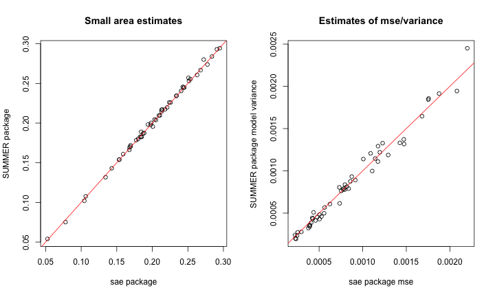
The SUMMER package includes functions to generate
additional diagnostic plots based on samples from the model posterior.
The compareEstimates() function generates a heatmap of the
posterior pairwise probabilities of one area’s mean exceeding another’s
mean.
When geographic polygon data for each domain is available as a
shapefile, the sf package can be used to load this data in
R. The mapEstimates() function can then be used to provide
a summary map of posterior medians or posterior variances.
Spatial Fay-Herriot
The sae package also provides tools for implementing a
spatial version of the Fay-Herriot model which assumes that the vector
of area specific effects follows a first order simultaneous
autoregressive, or SAR(1), process:
where
is the identity matrix for the
areas and
is a vector of zeroes of size
.
Additionally,
is an autoregression parameter and
is an adjacency matrix (with rows standardized to sum to 1).
The sae::mseSFH function estimates the unknown variance
parameters, the resulting EBLUP small area estimators, and then uses
bootstrap methods to estimate the MSE of the estimators.
To illustrate the use of this function, Molina
and Marhuenda (2015) consider a synthetic dataset concerning
grape production surface area for 274 Italian municipalities. Below we
load the relevant objects from the sae package. The
grapes dataset containes direct estimators of the mean
surface area in hectares for grape production in each municipality
(grapehect), the sampling variance of these direct
estimators (var), and relevant covariates including number
of working dats and overall agrarian surface area. The
grapesprox object contains the relevant adjacency matrix
representing the municipalities’ neighborhood structure.
Results using sae
sae.FH.grapes <- sae::mseSFH(grapehect ~ area + workdays - 1, var, grapesprox, data = grapes)

results <- data.frame(DIR = grapes$grapehect,
                      eblup.SFH = sae.FH.grapes$est$eblup,
                      mse = sae.FH.grapes$mse)
# reorder results for comparison later
results$area_name <- paste0('area_', rownames(results))
Results using SUMMER
The smoothArea function also allows the use of a model
with spatially correlated area effects, but the default implementation
assumes a BYM2 model for
rather than a simultaneous autoregressive model as in the SFH model
implemented in sae.
# create area_name as SUMMER requires rownames of adj.mat to match area variable
grapes$area_name <- paste0('area_', rownames(grapes))
adj.mat.grapes <- as.matrix(grapesprox)
rownames(adj.mat.grapes) <- colnames(adj.mat.grapes) <- grapes$area_name
X_grapes <- grapes[,c('area_name', 'area', 'workdays')]

# format direct estimates for SUMMER
grapes.dir <- grapes[, c(5, 1, 4)]
# scale direct estimates for use with INLA
grapes.dir$grapehect <- grapes.dir$grapehect / 10
grapes.dir$var <- grapes.dir$var/ 100
summer.FH.grapes <- smoothArea(formula = grapehect~area + workdays,
                               direct.est = grapes.dir, X.domain = X_grapes,
                               domain = ~area_name, adj.mat = adj.mat.grapes)
plot_list <- plot(summer.FH.grapes, return_list = T)
Despite the differing models, we again observe good agreement with the estimates, though less so with the estimates of uncertainty.
summer.bym2.est <-
  summer.FH.grapes$bym2.model.est[match(rownames(adj.mat.grapes), summer.FH.grapes$bym2.model.est$domain),]
par(mfrow = c(1, 2))
plot(results$eblup.SFH,
     summer.bym2.est$median * 10,
     xlab = "sae package",
     ylab = "SUMMER package",
     main = "Small area estimates")
abline(0, 1, col = 'red')
plot(results$mse,
     summer.bym2.est$var * 100,
     xlab = "sae package mse",
     ylab = "SUMMER package model variance",
     main = "Estimates of mse/variance")
abline(0, 1, col = 'red')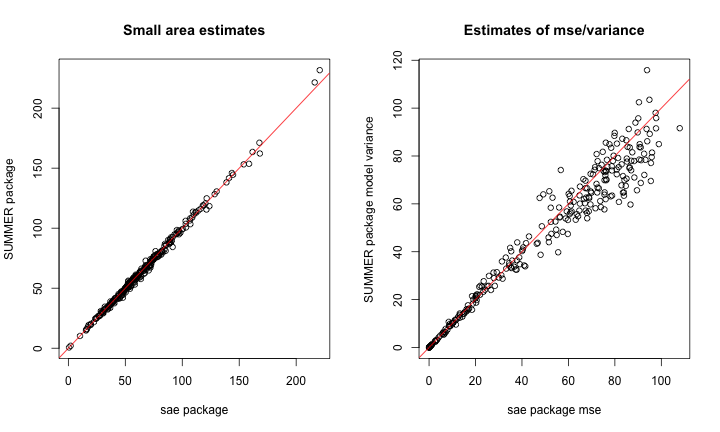
BRFSS Data
Below, we provide an example comparing spatial models from
sae and SUMMER using data from the Behavioral
Risk Factor Surveillance System (BRFSS).
library(ggplot2)
library(patchwork)
data(BRFSS)
data(KingCounty)
BRFSS <- subset(BRFSS, !is.na(BRFSS$diab2))
BRFSS <- subset(BRFSS, !is.na(BRFSS$hracode))
head(BRFSS)
##   age pracex       educau zipcode    sex street1 street2      seqno year
## 1  30  White college grad   98001   male      NA      NA 2009000041 2009
## 2  26  White college grad   98107 female      NA      NA 2009000309 2009
## 3  33  Black college grad   98133   male      NA      NA 2009000404 2009
## 4  25  White some college   98058   male      NA      NA 2009000531 2009
## 5  23  White some college   98102   male      NA      NA 2009000675 2009
## 6  19  Asian some college   98106   male      NA      NA 2009000694 2009
##   hispanic mracex strata             hracode tract rwt_llcp genhlth2 fmd obese
## 1 non-Hisp  White  53019        Auburn-North    NA 2107.463        0   0     0
## 2 non-Hisp  White  53019             Ballard    NA 2197.322        0   1     0
## 3 non-Hisp  Black  53019          NW Seattle    NA 3086.511        0   0     0
## 4 non-Hisp  White  53019        Renton-South    NA 3184.740        1   1     1
## 5 non-Hisp  White  53019 Capitol Hill/E.lake    NA 3184.740        0   0     0
## 6 non-Hisp  Asian  53019      North Highline    NA 4391.304        0   0     0
##   smoker1 diab2 aceindx2 zipout streetx ethn age4 ctmiss
## 1       0     0       NA  98001       0    1    3      1
## 2       0     0       NA  98107       0    1    3      1
## 3       0     0       NA  98133       0    2    3      1
## 4       0     0       NA  98058       0    1    3      1
## 5       0     0       NA  98102       0    1    4      1
## 6       0     0       NA  98106       0    3    4      1
mat <- getAmat(KingCounty, KingCounty$HRA2010v2_)
## Warning in spdep::poly2nb(geo, queen = F, row.names = names): some observations have no neighbours;
## if this seems unexpected, try increasing the snap argument.
## Warning in spdep::poly2nb(geo, queen = F, row.names = names): neighbour object has 2 sub-graphs;
## if this sub-graph count seems unexpected, try increasing the snap argument.
design <- svydesign(ids = ~1, weights = ~rwt_llcp,
                    strata = ~strata, data = BRFSS)
direct <- svyby(~diab2, ~hracode, design, svymean)
Results using sae
Below, we use sae to smooth the logit-transformed direct
estimates.
direct$var <- direct$se ^ 2
direct$logit.diab2 <- SUMMER::logit(direct$diab2)
direct$logit.var <- direct$var / (direct$diab2 ^ 2 * (1 - direct$diab2) ^ 2)
SFH.brfss <- sae::mseSFH(logit.diab2 ~ 1, logit.var, mat, data = direct)

results <- data.frame(domain = direct$hracode,
                      eblup.SFH = SUMMER::expit(SFH.brfss$est$eblup),
                      mse = SFH.brfss$mse)
Results using SUMMER
Below, we fit two versions of the spatial area levelmodel in
SUMMER. If we change pc.u and
pc.alpha from the default value
to
,
we assign more prior mass on smaller variance of the random effects,
inducing more smoothing.
summer.brfss <- smoothArea(diab2~1, domain= ~hracode,
                           design = design,
                           transform = "logit",
                           adj.mat = mat, level = 0.95)
summer.brfss.alt <- smoothArea(diab2~1, domain= ~hracode,
                               design = design,
                               transform = "logit",
                               adj.mat = mat, level = 0.95,
                               pc.u = 0.1, pc.alpha = 0.01)
Finally, we use SUMMER::mapPlot to compare median
estimates and uncertainty estimates obtained via sae and
SUMMER.
toplot <-  summer.brfss$bym2.model.est
toplot$logit.var <- toplot$var /
  (summer.brfss$bym2.model.est$median ^ 2 *
     (1 - summer.brfss$bym2.model.est$median) ^ 2)
toplot$median.alt <-  summer.brfss.alt$bym2.model.est$median
toplot$logit.var.alt <-  summer.brfss.alt$bym2.model.est$var /
  (summer.brfss.alt$bym2.model.est$median ^ 2 *
     (1 - summer.brfss.alt$bym2.model.est$median) ^ 2)
toplot$median.sae <- results$eblup.SFH
toplot$mse.sae <- results$mse
variables <- c("median", "median.alt",  "median.sae",
               "logit.var", "logit.var.alt", "mse.sae")
names <- c("Median (default prior)", "Median (new prior)",  "EBLUP (sae)",
           "Variance (default prior)", "Variance (new prior)", "MSE (sae)")
mapPlot(data = toplot, geo = KingCounty,
        variables=variables[1:3],
        labels = names[1:3], by.data = "domain",
by.geo = "HRA2010v2_", size = 0.1) 
mapPlot(data = toplot, geo = KingCounty,
        variables=variables[4:6], labels = names[4:6],
by.data = "domain", by.geo = "HRA2010v2_", size = 0.1) 
par(mfrow = c(1, 2))
range1 <- range(c(direct$diab2,toplot$median.alt))
plot(direct$diab2,toplot$median,
     xlab = "direct estimates",
     ylab = "model-based estimates",
     main = "Small area estimates", col = 'red', pch = 16,
     xlim=range1,ylim=range1)
points(direct$diab2,toplot$median.sae,  col = 'blue', pch = 16)
points(direct$diab2,toplot$median.alt,  col = 'cyan', pch = 16)
legend('topleft', pch = 16, col = c('red', 'cyan', 'blue'),
       legend = c("SUMMER",'SUMMER (new prior)', "sae"),bty="n")
abline(0,1)
range2 <- range(c(direct$logit.var,toplot$mse.sae,toplot$logit.var.alt))
plot(direct$logit.var,toplot$logit.var,
     xlab = "direct estimate var.",
     ylab = "model-based uncertainty",
     main = "Small area estimates", col = 'red', pch = 16,
     xlim=range2,ylim=range2)
points(direct$logit.var,toplot$mse.sae,  col = 'blue', pch = 16)
points(direct$logit.var,toplot$logit.var.alt,  col = 'cyan', pch = 16)
legend('topleft', pch = 16, col = c('red', 'cyan','blue'),
       legend = c("SUMMER var.", 'SUMMER var. (new prior)', "sae mse"),bty="n")
abline(0,1)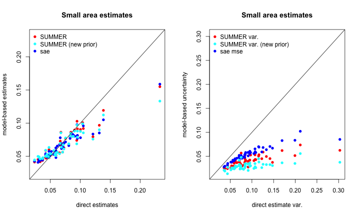
Unit Level Models
The nested error model, introduced by Battese, Harter, and Fuller (1988), uses auxiliary data at the unit level.
Nested error model:
Here are area random effects and are unit level errors. This model assumes the sampling design is ignorable.
The sae package conducts estimation of domain means by
first estimating variance parameters
and
.
Next, given known variance parameters, domain means
are predicted by calculating the EBLUPs.
The area fitted values are: where
is the domain sampling fraction.
is the mean response in the sampled units.
is the mean of the covariates in the sampled units.
is the mean of the covariates in the population.
is the estimated random effect.
Corn and Soy Production
The cornsoybean and cornsoybeanmeans
datasets contain info on corn and soy beans production in 12 Iowa
counties Battese, Harter, and Fuller
(1988). The objective here is use satellite imagery of the number
of pixels assigned to corn and soy to estimate the hectares grown of
corn.
-
SampSegments: sample size. -
PopnSegments: population size. -
MeanCornPixPerSeg: county mean of the number of corn pixels (satellite imagery). -
MeanSoyBeansPixPerSegcounty mean of the number of soy beans (satellite imagery) pixels.
The variables MeanCornPixPerSeg and
MeanSoyBeansPixPerSeg provide the known county means of the
auxiliary variables.
We load the sample data:
##   County CornHec SoyBeansHec CornPix SoyBeansPix
## 1      1  165.76        8.09     374          55
## 2      2   96.32      106.03     209         218
## 3      3   76.08      103.60     253         250
## 4      4  185.35        6.47     432          96
## 5      4  116.43       63.82     367         178
## 6      5  162.08       43.50     361         137
Next, we load the population auxiliary information:
data("cornsoybeanmeans")
Xmean <-
  data.frame(cornsoybeanmeans[, c("CountyIndex",
                                  "MeanCornPixPerSeg",
                                  "MeanSoyBeansPixPerSeg")])
head(Xmean)
## CountyIndex MeanCornPixPerSeg MeanSoyBeansPixPerSeg
## 1 1 295.29 189.70
## 2 2 300.40 196.65
## 3 3 289.60 205.28
## 4 4 290.74 220.22
## 5 5 318.21 188.06
## 6 6 257.17 247.13
Popn <-
  data.frame(cornsoybeanmeans[, c("CountyIndex",
                                  "PopnSegments")])
head(Popn)
## CountyIndex PopnSegments
## 1 1 545
## 2 2 566
## 3 3 394
## 4 4 424
## 5 5 564
## 6 6 570The sae::pbmseBHF function obtains EBLUPs under the
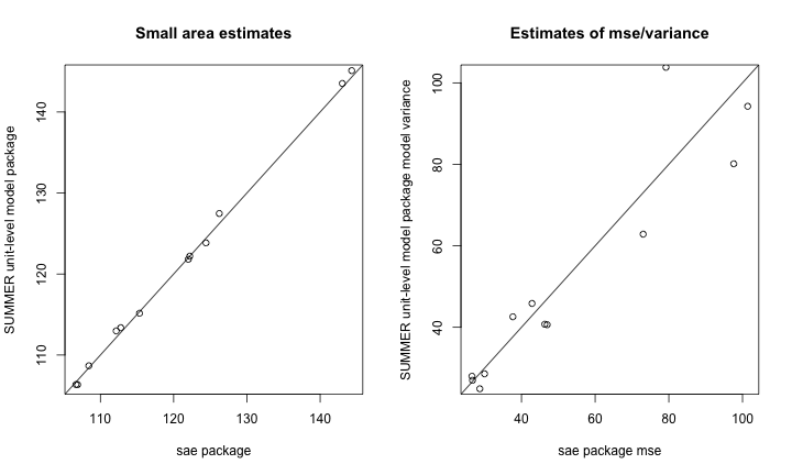
nested error model and then uses a parametric bootstrap approach to
estimate MSEs.
cornsoybean <- cornsoybean[-33, ] # remove outlier
sae.bhf <-
  pbmseBHF(CornHec ~ CornPix + SoyBeansPix,
           dom = County, meanxpop = Xmean,
           popnsize = Popn, B = 200,
           data = cornsoybean)
SUMMER::smoothUnit provides the ability to fit unit
level models with unit level covariates for Gaussian response variables.
Below we use the is.unit argument to specify a unit level
model and then provide the column names of the unit level covariates in
X.unit. Finally, the X argument provides the
area level means of each covariate for use when generating predictions.
Note that in order to align the SUMMER estimates with those
from the sae package, we specify a relatively flat prior on
the variance of the area-specific random effect
(pc.u = 100, pc.alpha = 0.01 specifies a penalized
complexity prior such that
where
is the standard deviation of the area-specific random effects).
cornsoybean$id <- 1:dim(cornsoybean)[1]
Xsummer <- Xmean
colnames(Xsummer) = c("County", "CornPix", "SoyBeansPix")
des0 <- svydesign(ids = ~1, data = cornsoybean)
## Warning in svydesign.default(ids = ~1, data = cornsoybean): No weights or
## probabilities supplied, assuming equal probability
summer.bhf.unit <- smoothUnit(formula = CornHec ~ CornPix + SoyBeansPix,
                              family = "gaussian",
                              domain = ~County,
                              design = des0, X.pop = Xsummer,
                              pc.u = 1000, pc.alpha = 0.01, level = 0.95)
## Warning in smoothUnit(formula = CornHec ~ CornPix + SoyBeansPix, family =
## "gaussian", : No spatial information provided, using iid domain effects
Below, we plot comparisons of the sae and
SUMMER results.
par(mfrow = c(1, 2))
range1 <- range(c(sae.bhf$est$eblup$eblup,summer.bhf.unit$median))
plot(sae.bhf$est$eblup$eblup,summer.bhf.unit$iid.model.est$median,
     xlab = "sae package",
     ylab = "SUMMER unit-level model package",
     main = "Small area estimates",
     xlim=range1,ylim=range1)
abline(0,1)
range2 <- range(c(sae.bhf$mse$mse, summer.bhf.unit$var))
plot(sae.bhf$mse$mse, summer.bhf.unit$iid.model.est$var,
     xlab = "sae package mse",
     ylab = "SUMMER unit-level model package model variance",
     main = "Estimates of mse/variance",
     xlim=range2,ylim=range2)
abline(0,1)